Model Accuracy Evaluation
About model accuracy evaluation
Definition
- What it does: Model accuracy evaluation verifies the prediction accuracy of your custom inference implementation (written per this document) on a given dataset.
- Requirement: The model inference service must be reachable via the streaming API at
/v1/chat/completions.
How to run an accuracy evaluation
- Write your script following the “Model accuracy evaluation run script” section below. Note: Only the model adapter repository admin can start an accuracy evaluation, and the repository hardware type must be NPU.

- Open the Model evaluation tab and go to the model evaluation page.
- On the model accuracy page, open the Accuracy tab, select the model weights repository, then click Run test to start the evaluation.

- Wait until the accuracy run finishes.

- (Optional) While status is Running, you can click Stop test to cancel.
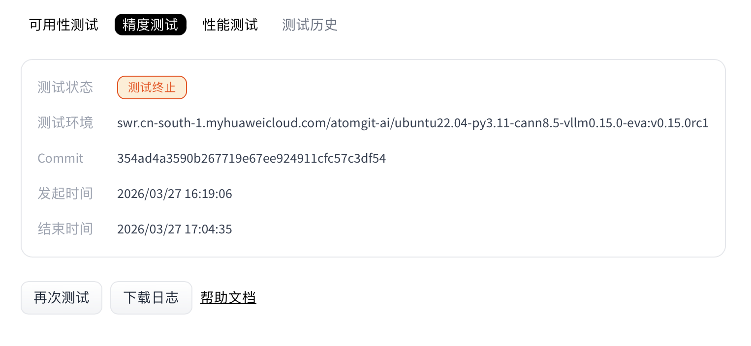
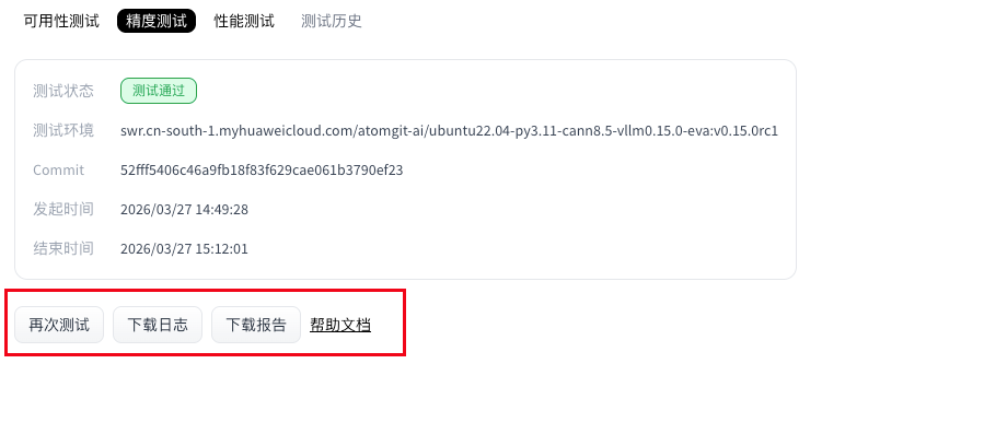
- When the run completes, the Accuracy section shows status and provides logs and report downloads.
Model accuracy evaluation run script
Accuracy evaluation uses deploy.sh as the entry point. Follow this document strictly when writing scripts.
The adapter repository for accuracy evaluation must include:
requirements.txt: Python packages needed to run the script. Omit this file if there are no extra dependencies (optional).deploy.sh: The evaluation service uses this script to install dependencies and start the adapter project (required).
File locations
requirements.txt and deploy.sh must be at the repository root.
requirements.txt (optional)
List NPU-side dependencies required to run the script. Torch NPU, CANN, and Python are provided by the environment for the selected framework version—do not duplicate them in requirements.txt (that can cause install conflicts). Example:
transformers==4.37.0
accelerate==0.27.2
If you need no extra packages, you may omit the .txt file; the job skips dependency installation.
deploy.sh
This shell script starts model adapter inference; how you run inference inside is flexible. Conventions below apply.
Example: install dependencies (optional)
python3 -m pip install --upgrade pip setuptools wheel
Passing parameters into the script
Weights are downloaded at test time from the repository you selected when starting the evaluation. To pass the weight path in the shell script, use the environment variable $MODEL_PATH (path to the weight files). Example for launching with vLLM:
vllm serve "$MODEL_PATH" --trust-remote-code --tensor-parallel-size 1 --dtype float16 --max-num-seqs 4 --gpu-memory-utilization 0.95
Adapter code requirements
Inference must expose a standard OpenAPI-compatible inference API, and the HTTP server must listen on port 8000. The evaluation service calls the matching inference API for the selected weights’ task type. Supported task types:
| Task type | Task code | Inference API path |
|---|---|---|
| Text generation | text-generation | /v1/chat/completions |
| Image to text | image-text-to-text | /v1/chat/completions |
| Multimodal | any-to-any | /v1/chat/completions |
Note: Accuracy evaluation relies on
/v1/chat/completions. If that endpoint is missing, the accuracy job fails.
Model weight size limit
- Maximum size: 100 GB
- Rule: Adapter weight storage must not exceed this limit.
- If exceeded: Weight download fails and the accuracy job fails.
End-to-end example
deploy.sh
- vLLM adapter example:
#!/bin/sh
set -e
echo "=== MODEL_PATH set to: $MODEL_PATH ==="
vllm serve "$MODEL_PATH"  --trust-remote-code --tensor-parallel-size 1 --dtype float16   --max-num-seqs 4  --gpu-memory-utilization 0.95
Note: In this vLLM example you do not need
--served-model-name; the evaluation service uses the weight path as the served model name automatically.
Accuracy report
After a successful run, download and unzip the accuracy report. It contains the folders configs, predictions, results, and summary.
Directory layout:
ee9480acbbac4d4aa190a124d5ddf39c/
├── configs # Combined config from model task, dataset task, and presentation task
│   └── 20260326_151326_29317.py
├── logs # Runtime logs; with --debug in the command, step logs go to stdout only
│   ├── eval
│   │   └── vllm-api-general-chat
│   │       └── demo_gsm8k.out # Accuracy-evaluation log from predictions/
│   └── infer
│       └── vllm-api-general-chat
│           └── demo_gsm8k.out # Inference log
├── predictions
│   └── vllm-api-general-chat
│       └── demo_gsm8k.json # Model outputs (full responses from the service)
├── results
│   └── vllm-api-general-chat
│       └── demo_gsm8k.json # Raw scores from accuracy metrics
└── summary
    ├── summary_20260326_151326.csv # Final scores (CSV)
    ├── summary_20260326_151326.md # Final scores (Markdown)
    └── summary_20260326_151326.txt # Final scores (plain text)
Example content of summary/summary_20260326_151326.md:
| dataset | version | metric | mode | vllm-api-stream-chat |
|---|---|---|---|---|
| demo_gsm8k | 0ba9da | accuracy (5 runs average) | gen | 5.60 |
| demo_gsm8k | 0ba9da | avg@5 | gen | 5.60 |
| demo_gsm8k | 0ba9da | pass@5 | gen | 24.00 |
| demo_gsm8k | 0ba9da | cons@5 | gen | 0.00 |
Interpreting accuracy results
I. Relationship among n, k, and num_return_sequences in the API config
1. How pass@k is computed
This section only sketches
pass@k; for other metrics see Definitions and relationships of pass@k, cons@k, and avg@n.
pass@k is a core metric for code generation: the probability that at least one of k sampled candidates passes all tests. It uses an unbiased estimator to avoid high variance from naive sampling. Steps:
Samples and correctness
- For each problem, generate
ncandidates (n ≥ k);cof them pass tests. - Example:
n = 100samples,c = 20correct—per-sample pass rate follows from that.
- For each problem, generate
Combinatorial form
- Probability that a random
k-subset of thensamples is all wrong:
$$ pass@k = 1 - \frac{\binom{n-c}{k}}{\binom{n}{k}} $$pass@kis one minus that (at least one success):Stable implementation: to avoid factorial overflow, code uses:
pass@k = 1 - np.prod(1.0 - k / np.arange(n - c + 1, n + 1))- Probability that a random
Why unbiased estimation
In the current implementation,
kandnare tied tonum_return_sequencesonly; this section highlights why the unbiased form helps.Sampling
ktimes directly has high variance (especially for largek); generatingnwithn >> kand using the combinatorial formula improves stability. Example:n = 5,c = 3,k = 2:P(all wrong in a random pair) =
C(2,2)/C(5,2) = 1/10 = 0.1pass@2 = 1 - 0.1 = 0.9(90% chance at least one success in two tries).
2. How n, k, and num_return_sequences relate
All three must be positive integers. The accuracy service defaults
num_return_sequencesto 5.
| Configurable? | Parameter | Meaning | Where defined | Constraints |
|---|---|---|---|---|
| No | n | Number of rollouts per problem (total generated samples) | Not separately configurable; equals num_return_sequences | Requires n ≥ k; no separate n today |
| No | k | Sample size for evaluation; scales pass@k | Not separately configurable; equals num_return_sequences | Same as above |
| Yes | num_return_sequences | Independent repeated completions per request | API model config; default 5 | — |
3. Summary
pass@k: Unbiased combinatorial estimate; reduces variance of naive sampling.- Current constraints:
nandkare not independently configurable—onlynum_return_sequencesin the API config matters.n=k=num_return_sequences- The
kornin names likepass@k,cons@k,avg@nall refer tonum_return_sequences
nandkare only used at evaluation time, whilenum_return_sequencesdrives inference—but values come from the API config. When running evaluation (--mode eval), ensure reused inference outputs were produced with the samenum_return_sequencesas the current setting.
II. Definitions and relationships: pass@k, cons@k, avg@n
1. Background
In LLM and multimodal RL evaluation, pass@k, cons@k, and avg@n summarize multi-sample behavior from different angles. They suit tasks that need multiple independent attempts (code, math, RL, etc.) and give statistically meaningful views of performance.
2. Definitions and computation
2.1 Definitions
Formal definitions:
pass@k:
$$ 1 - \prod_{j=n-c+1}^{n} (1 - \frac{k}{j}) $$ cons@k:
$$ \frac{1}{N} \sum_{i=1}^{N} I(c_i > k/2) $$ avg@n:
$$ \frac{1}{N} \sum_{i=1}^{N} \frac{c_i}{n} $$| Metric | What it measures | Goal | Range |
|---|---|---|---|
| pass@k | P(at least one correct) (unbiased) | Reliability of solving | [0, 1] |
| cons@k | Majority-correct rate | Stability of outputs | [0, 1] |
| avg@n | Mean per-sample accuracy | Overall correctness | [0, 1] |
Where:
- N: Total number of problems in the dataset.
- n: Rollouts per problem (total samples), matching code parameter
n. - k: Evaluation sample size for
pass@kandcons@k, matching code parameterk. - cᵢ: Number of correct samples for problem i.
- I(·): Indicator (1 if condition holds, else 0).
- Product index j runs from
n - c + 1tonfor numerical stability.
2.2 Details
pass@k: Unbiased estimator; implemented ascompute_pass_at_k(n, c, k)wherenis total samples,ccorrect count,ksample size—algebraically equivalent to the binomial form but implemented in product form.cons@k: “Consistency” / stability—share of problems where a strict majority of samples are correct. Per problem, count 1 if correct count >k/2, else 0; average over problems (majority-vote style).avg@n: Mean over problems ofc / n(per-problem accuracy); reflects overall sample-level correctness.
2.3 Example (num_return_sequences = 3, so n = k = 3)
Problem 1: preds [A, A, X] → c = 2
Problem 2: preds [B, C, B] → c = 2
Problem 3: preds [X, X, C] → c = 1
Problem 4: preds [X, X, X] → c = 0

pass@3 = (1.0 + 1.0 + 1.0 + 0.0)/4 = 0.75 (at least one correct on 1–3; none on 4)
avg@3 = (2/3 + 2/3 + 1/3 + 0/3)/4 ≈ 0.4167
cons@3 = (1 + 1 + 0 + 0)/4 = 0.5 (majority correct on 1–2; not on 3–4)
3. cons@k vs avg@n
3.1 Ordering
By construction,
pass@kis always ≥ bothavg@nandcons@k—it cannot be smaller—so we do not comparepass@kto the other two here.
The ordering of cons@k and avg@n depends on prediction patterns.
Case 1: cons@k > avg@n
- Pattern: Highly consistent but not perfect (many problems have a strict majority correct, yet not 100% per-sample accuracy).
- Example:
k = 3, two problems:- P1:
[A, A, B], goldA→c = 2, rate ≈ 0.667; majorityA(2 > 1.5) → cons contributes 1. - P2:
[B, B, C], goldB→ same; cons contributes 1. avg@n= (0.667 + 0.667) / 2 = 0.667cons@k= (1 + 1) / 2 = 1.0- So
cons@k>avg@n.
- P1:
Case 2: cons@k < avg@n
- Pattern: Predictions spread out—no majority—but average correctness can still be moderate (correctness spread thin).
- Example:
k = 3, two problems:- P1:
[A, B, C], goldA→c = 1, rate ≈ 0.333; no strict majority → cons 0. - P2:
[A, B, C], goldB→ same → cons 0. avg@n= 0.333cons@k= 0- So
cons@k<avg@n.
- P1:
Case 3: cons@k ≈ avg@n
- Pattern: Near-perfect or all-wrong, or distributions where majority rate tracks mean rate.
- Example:
k = 3, two problems:- P1:
[A, A, A], goldA→ rate 1.0; majority correct → cons 1. - P2:
[B, B, B], goldC→ rate 0.0; majority wrong → cons 0. avg@n= 0.5cons@k= 0.5- So
cons@k=avg@n.
- P1:
3.2 Trends
- High agreement (strict majorities often correct) can push
cons@kaboveavg@nbecause cons only needs a majority while mean is dragged by errors. - Spread predictions without majorities can make
avg@nexceedcons@k(partial credit vs majority rule). - At extremes (all right or all wrong), the two often align.
- In practice (e.g. multi-turn RL), use
cons@kfor stability andavg@nfor overall accuracy—they complement each other; no fixed ordering.
4. Takeaways
Which metric when
pass@k: Model potential / best-effort successcons@k: Stabilityavg@n: Aggregate sample accuracy
Common pitfalls
- Only
pass@1: Ignores multi-try capability - Ignoring
cons@k: May hide instability in production avg@nalone: Cannot separate consistency vs fault tolerance
- Only
Heuristic thresholds and decisions
Thresholds below are illustrative: high (>0.8), mid (0.5–0.8), low (<0.5). Use as guidance only.
Scenario guide
Scenario Primary Secondary Targets Reliability-first (medical, finance) cons@k pass@k cons@k > 0.8, pass@k > 0.9 Fault-tolerance-first (code, exploration) pass@k avg@n pass@k > 0.8, avg@n > 0.7 Balanced (general assistant) avg@n cons@k + pass@k avg@n > 0.75 Decision matrix
Profile Situation Next steps High pass@k, mid avg@n, low cons@k Strong but unstable Improve consistency (temperature, voting) Mid across all Even but mediocre Broad improvements (data, prompts) Low pass@k & avg@n, high cons@k Systematic bias Audit data, prompts, model bias All low Failing Retrain or change architecture
Using all three together gives a fuller picture for tuning and deployment.
5. Caveats
Not every dataset config’s Evaluator implements all three metrics. If eval_cfg points to an evaluator that does not return the needed quantities, the UI falls back to the original accuracy-style metrics only.
Source for the above: AISBench documentation.